Psychology 105
Richard Lowry
©1999-2002

Some Basic Statistical Concepts and Methods
for the Introductory Psychology Course
Part 3


Measures of Central Tendency

   Potentially, you could have two quite different types of measures of central tendency. The first would measure the strength of the tendency for measures to cluster together, and the second would measure the location where the clustering tends to occur. Typically when we speak of measures of central tendency, it is the second type of measure that we are talking about—the measure of location. The measure of the strength of the tendency, on the other hand, is actually the flip-side of the measures of variability that we will be examining in the section that follows this one.

   The three most commonly used measures of the location of central tendency are the mode, the median, and the mean. In brief, the mode is the point or region within a distribution where the largest number of individual measures congregate, the median is the midpoint of all the individual measures, and the mean is the arithmétic average of all the individual measures.

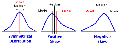
   As a rule, the only time you will find the mode and median to be precisely coincident with the mean is when the distribution is unimodal and perfectly symmetrical. In skewed distributions the mean, median, and mode will tend to be separated from one another, with the mean falling toward the tail of the skew, the mode falling away from the tail, at the peak, and the median falling somewhere in-between. Thus, in a positively skewed distribution the mean will be to the right, the mode to the left, and the median in-between, while in a negatively skewed distribution the mean will be to the left, the mode to the right, and the median in-between. These relationships among the three measures of central tendency are shown below in Figure 3.1.

Figure 3.1. Relationships of the Mean, Median, and Mode in Symmetrical and Skewed Distributions

   If your purposes in assessing the central tendency of a distribution are purely descriptive, your best procedure would be to examine not just the mode or the median or the mean separately, but all three together. But once you step beyond those limited purposes into the much broader realm of analytical and inferential statistics, the mode and the median become virtually useless The reason for this is that measures of mode and median do not have the properties of an equal interval scale of measurement—this is true even if the data on which they are based do have the properties of an equal interval scale—hence they cannot meaningfully be subjected to any further mathematical operations. In brief, they are both mathematical dead ends. The mean, on the other hand, providing it is based on data that derive from an equal interval scale of measurement, will itself have the properties of an equal interval scale and thus can be subjected to further mathematical operations.

   The arithmétic mean of a distribution is simply the sum of all the values in the distribution divided by the number of values. Thus, the mean of a distribution consisting of the values 1, 2, 3, 4, and 5 is
mean =
sum of all values
number of values
 
=
1 + 2 + 3 + 4 + 5
5
=
15
5
= 3.0

   You can think of the mean as the balance point within a distribution, a kind of center of gravity to which each measure in the distribution contributes in proportion to its size. Thus a distribution consisting of the values 1, 2, 2, and 3 would balance, as shown below, at (1+2+2+3)/4 = 2.0.


Replace any of the four values in this distribution with some other value, and the balance point shifts accordingly. In the following illustration we replace the 3, first with a 5 and then with a 9. For the first replacement the balance point shifts from 2.0 to 2.5, and for the second it shifts even further to 3.5.


And please take special note of the tidy proportionality of these shifts. In this particular distribution there are four values, each contributing 1/4 = 25% to the determination of the mean. Increase any particular value by one point (one unit of measurement), and you will increase the mean by 0.25 units; increase the value by two points, and you will increase the mean by 0.50 units; and so on. Conversely, decrease any value in the distribution by a certain amount and you will decrease the mean by 25% of that amount. In a distribution composed of three values, the contribution of each individual value would be 1/3 = 33.3%; in one composed of 10 values it would be 1/10 = 10%; and so on.

   And now for a formula and an introduction to some conventional statistical notation. When you calculate the mean of a distribution you are performing two separate computational steps: first, you are taking the sum of all the individual values in the distribution; and then you are dividing that sum by the total number of values in the distribution. In the formulaic description of these two steps that we gave earlier, notice that the second step is expressed not in words but by an abstract symbol:
mean =
sum of all values
number of values
The horizontal line between "sum of all values" and "number of values" is a conventional, concise symbolic way of saying something that would otherwise be very cumbersome to say, especially if it needed to be said over and over again in a variety of different situations: namely, "take whatever is above the line and divide it by whatever is below it." As it happens, you have a very long-standing familiarity with this particular symbolic notation, as you do with its substitutes "÷" and "/ ", as well as with its cousins "+", "", and "x", and so your eye and mind see immediately precisely what operation it is telling you to perform. The formula that follows replaces each of the other terms and operations involved in the calculation of the mean with symbols that are equally concise. Please do not be intimidated by these symbols, for there is nothing at all elusive or arcane about them. It is simply a matter of familiarization. After a while their meanings will leap out at you as though you had been using them all your life.


Formula for the Calculation of the Arithmétic Mean

¶Definition of Terms
   N   
= the number of individual values in the distribution.
Xi
This is a symbol referring to the N individual values of your distribution in the abstract. Each value in the distribution is spoken of as a variate instance of the variable X. Thus, the first value in the distribution would be X1; the second would be X2; and so on to the last value, XN.

This symbol (upper-case Greek letter 'sigma') does not represent a numerical value, but rather, like "+" and "", a mathematical operation that is to be performed upon certain designated numerical values. It is a computational signpost saying "calculate the sum of these values"; hence its conventional name, the summation sign. Thus for a distribution of size N = 4, consisting of the values 6, 9, 12, and 15, the expression Xi would be equivalent to 6+9+12+15 = 42.
M
We will use the bold-face letter M to represent the arithmétic mean of a distribution. Thus MX would be the mean of a set of X values, MY would be the mean of a set of Y values, and so on. [Note that hardcopy statistics textbooks will often represent the mean of X (Y, Z, etc.) by writing the letter X (Y, Z, etc.) with a horizontal bar over it.]


¶FormulaT
mean =
sum of all values
number of values

Substitute the symbolic expressions for the verbal phrases in this structure, and you haveT
MX = Xi
TNT

   The best way to get a feeling for what a formula does is to apply it to a specific numerical example. Here again is the distribution of 12 exam scores mentioned earlier.
X1 X2 X3 X4 X5 X6 X7 X8 X9 X10 X11 X12
61 69 72 76 78 83 85 85 86 88 93 97
Add these N = 12 scores together and you will find that their sum comes out to 973. Substitute this value into the formula for the mean, and you haveT
MX =
Xi
TNT
=
973
12
= 81.08

   It is as simple as that.

   Actually, the value of the mean that you would calculate in this example would not come out to precisely 81.08, but rather to 81.08333... . Almost always when you calculate a mean you will end up having to do some rounding. However, do be careful not to round it down too much, because the mean often enters into subsequent calculations that can be thrown considerably askew if it is rounded excessively. In general, it is good practice to calculate the mean out to at least one decimal place beyond the number of decimal places contained in the original data. Thus, if the original data have no decimal places, as in the present example, carry the mean out to at least one decimal place; if they have one decimal place, carry it out to two; if they have two decimal places, carry it out to three; and so on.


Go to Part 4 [Measures of Variability]