Psychology 105
Richard Lowry
©1999-2002

Some Basic Statistical Concepts and Methods
for the Introductory Psychology Course
Part 4


Measures of Variability

   One very easy measure of the variability that exists within a distribution is the range, which is simply the distance between the lowest score in the distribution and the highest. Equally easy is the interquartile range, which is the distance between the lowest and highest of the middle 50 percent of the scores in the distribution. Thus for our 12 exam scores, the range extends from a low of 61 to a high of 97, and the interquartile range extends from a low of 76 to a high of 86.

Measures of this general type, however, are basically mathematical dead ends. They have a limited application for purely descriptive purposes, but beyond that there is very little you can do with them.

   Two somewhat more complex measures of variability that you can do something with are the variance and standard deviation, which go together like hand and glove, or more precisely, like square and square root. In brief, the variance is the square of the standard deviation, and the standard deviation is the square root of the variance.

variance = (standard deviation)2
standard deviation = sqrt[variance]

Note: Owing to the limitations of HTML coding for a web document, we will not be able to use the conventional radical sign to indicate "square root of." We will instead be using the notation "sqrt." Thus sqrt[variance] means "the square root of the variance," sqrt[16] means 'the square root of 16," and so forth.
   They are both ways of measuring variability, based on the realization that the dispersion within a distribution—the overall amount by which the individual values of Xi differ among themselves—is in direct proportion to the aggregate amount by which they differ or deviate from their collective mean. For each particular value of Xi within a distribution, the distance between it and the mean can be arrived at through a simple process of subtraction. By convention, Xi is placed to the left of the subtraction sign, the mean is placed to the right, and the result of the operation is spoken of as a deviate (noun). Thus

deviate = Xi MX

   In and of themselves, these deviate measures are useless as an aggregate measure of variability, because they will always sum up to zero (within the limits of rounding errors), no matter how much or little variability the distribution might actually contain. The way to get around this sum-to-zero problem is to take each deviate score and square it. Then add up all the squared deviates to arrive at a quantity known as the sum of squared deviates, conveniently abbreviated as SS.

squared deviate = (Xi MX)2
sum of squared deviates: SS = (Xi MX)2

The quantity calculated as SS will come out to zero only when the actual amount of variability within the distribution is zero. In all other cases it will come out as something larger than zero, in an amount precisely determined by the degree of variability that actually exists within the distribution.

   The variance is then simply the average of the squared deviates, and the standard deviation is the square root of that average. [But note the special caution below.] By convention, the variance and standard deviation of a distribution are symbolized as s2 and s, respectively. Thus

¶variance:
s2 = (Xi MX)2
N
= SS
N

¶standard deviation:

s = sqrt
[ (Xi MX)2
N
] = sqrt
[ SS
N
]

An Important Caution Concerning the Calculation of Variance and Standard Deviation
Textbooks in statistics will often use N-1 in the denominator of the formulas for the variance and standard deviation, rather than simply N, as I have done. Therein hangs a tale. The formulas that I have given, which use N in the denominator, provide the actual, unadorned, plain-vanilla variance and standard deviation for any particular set or sample of Xi values. When you use N-1 in the denominator, what you are actually doing is using the particular sample of Xi values to estimate the variance and standard deviation of the entire population of Xi values from which the particular sample comes. If you ever take a full-blown course in statistics, you will that the technical reasons for this substitution derive from the theory of probability. The technical distinction between samples and populations will be explained in Part 5 of this booklet.

   Thus, for a simple distribution consisting of the Xi values 1, 2, 3, 4, and 5:

Xi
deviate =
(Xi MX)
squared
deviate
(Xi MX)2
sum of squared deviates:
   SS = 10
variance:
   s2 = SS/N = 10/5 = 2
standard deviation:
   s = square_root(variance)
      = square_root(2)
     = +1.41
1
2
3
4
5
13 = 2
23 = 1
33 = 0
43 = +1
53 = +2
4
1
0
1
4
sum =
10


   You will sometimes find the variance (s2) referred to as the mean square, and the standard deviation (s) referred to as the root mean square. The former is a shorthand way of saying "the mean of the squared deviates," which is what the variance basically is, and the latter is a shorthand way of saying "the square root of the mean of the squared deviates," which is what the standard deviation basically is.

   At any rate, once you know the values of N and SS for a distribution, the remaining calculations for variance and standard deviation are utterly simple and straightforward. The only potential complexity is that it will often prove rather laborious to calculate the value of SS using the formula I have just given you:
SS = (Xi MX)2
This construction is typically spoken of as a conceptual formula, since it allows you to see the structure of exactly what you are doing when you calculate SS. In effect it is saying: take the difference between each value of Xi and the mean of the distribution, square each of those differences, and then add them all up.

   Obviously this structural visibility is an advantage for anyone who is just starting out in statistics, for it helps to keep the underlying logic of the calculation clearly in view. But it also has the disadvantage that it can be quite tedious and cumbersome to use in actual practice. In the calculation of SS, and thus of the variance and standard deviation, it is often preferable to use the following computational formula. In general, a computational formula is one that is algebraically equivalent to, and hence yields the same result as the corresponding conceptual formula, more easily, though without the advantage of clearly showing the underlying logic of the calculation. Incidentally, this computational formula for SS will also do the job more precisely, since it minimizes rounding errors. First some additional items of symbolic notation:

Xi2
The square of any particular value of Xi within the distribution. If Xi = 3, then Xi2 = 3x3 = 9; if Xi = 4, then Xi2 = 4x4 = 16; and so on.
Xi2
The sum of all the squared Xi values within the distribution. If the values of Xi within a distribution are 3, 4, and 5, the sum of the squared Xi values is Xi2 = 32+42+52 = 9+16+25 = 50.
Xi
The sum of the original (unsquared) values of Xi within a distribution. If the values of Xi within a distribution are 3, 4, and 5, the sum of the original (unsquared) squared Xi values is simply Xi = 3+4+5 = 12.
(Xi)2
The square of the value of Xi. That is, calculate the sum of the original (unsquared) values of Xi within the distribution, and then square that sum. For a distribution consisting of the Xi values 3, 4, and 5, (Xi)2 is equivalent to (3+4+5)2 = 122 = 144. Please note very carefully that (Xi)2 is not the same thing as Xi2. For (Xi)2 you are summing up all the original values of Xi and then squaring that sum, while for Xi2 you are squaring each individual value of Xi and then taking the sum of all those squared values.

   And then the formula:
SS = Xi2
(Xi)2
2N2

Thus, for our distribution of 12 exam scores:

Xi Xi2
sum of squared deviates:
    = 80,063 [(9732)/12]
    = 80,063 78894.08
    = 1168.92
variance:
  s2 = 1168.92/12 = 97.41
standard deviation:
  s = sqrt[variance]
     = sqrt[97.41]
     = +9.87
61
69
72
76
78
83
85
85
86
88
93
97
3721
4761
5184
5776
6084
6889
7225
7225
7396
7744
8649
9409
Sums Xi=
973
Xi2=
80,063


   Although the variance and standard deviation are equally valid measures of variability, the standard deviation is by far the more easily visualized and intuitively comprehended, because it is the one that is expressed in the same units of measurement as the original values of Xi of which the distribution is composed. When you calculate the standard deviation of our distribution of exam scores, the resulting value of s also refers to the scale of exam scores. The variance (s2), on the other hand, would refer to squared exam scores, which do not readily lend themselves to graphic representation nor intuitive understanding. This is not to suggest that the variance is inferior. It is, in fact, a very useful measure of variability in its own right, and in some respects it is even more useful than the standard deviation, notwithstanding that one cannot easily draw a picture of it. But that is a point best saved until later.

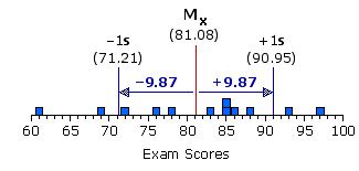
   At any rate, as we have just calculated, our distribution of exam scores has a standard deviation of s = +9.87. Figure 4.1 will give you an idea of what this rather abstract quantity—"plus or minus 9.87"—is saying about the distribution. Recalling that the mean of the distribution is 81.08, move one standard deviation to the right of the mean (MX+1s), and you end up at 81.08+9.87 = 90.95 on the exam-point scale. Move one standard deviation to the left of the mean (MX1s), and you end up at 81.089.87 = 71.21. For many types of distributions, the range between +1 and 1 standard deviation tends to encompass about two-thirds of all the individual values of Xi. Within the present distribution it is exactly two-thirds.

Figure 4.1. Graphic Representation of +1 and 1 Standard Deviation


   In effect, "plus or minus" one standard deviation represents a range within the distribution, centered upon the mean. Unlike the analogous interquartile range, however, the range between 1s and +1s is a measure of variability defined by all of the values of Xi within the distribution, each in proportion to its distance from the mean of the distribution. Thus, a compact distribution will have a relatively narrow range between 1s and +1s, while a more dispersed distribution will have a wider range, in proportion to the degree of its dispersion. Either way, you can in general expect approximately two-thirds of the values of Xi within a distribution to fall within the range between 1s and +1s, providing the distribution is not extremely skewed. For an extremely skewed distribution, it will tend to be more than two-thirds.


Go to Part 5 [Varieties of Distributions]