Psychology 105
Richard Lowry
©1999-2002

Some Basic Statistical Concepts and Methods
for the Introductory Psychology Course
Part 7


The Measurement of Linear Correlation

   The primary measure of linear correlation is the Pearson product-moment correlation coefficient, symbolized by the lower-case Roman letter r, which ranges in value from r=+1.0 for a perfect positive correlation to r=1.0 for a perfect negative correlation. The midpoint of its range, r=0.0, corresponds to a complete absence of correlation. Values falling between r=0.0 and r=+1.0 represent varying degrees of positive correlation, while those falling between r=0.0 and r=1.0 represent varying degrees of negative correlation.

   A closely related companion measure of linear correlation is the coefficient of determination, symbolized as r2, which is simply the square of the correlation coefficient. The coefficient of determination can have only positive values ranging from r2=+1.0 for a perfect correlation (positive or negative) down to r2=0.0 for a complete absence of correlation. The advantage of the correlation coefficient, r, is that it can have either a positive or a negative sign and thus provide an indication of the positive or negative direction of the correlation. The advantage of the coefficient of determination, r2, is that it provides an equal interval and ratio scale measure of the strength of the correlation. In effect, the correlation coefficient, r, gives you the true direction of the correlation (+ or ) but only the square root of the strength of the correlation; while the coefficient of determination, r2, gives you the true strength of the correlation but without an indication its direction. Both of them together give you the whole works.

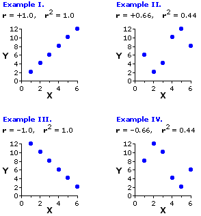
   We will examine the details of calculation for these two measures in a moment, but first a bit more by way of introducing the general concepts. Figure 7.1 shows four specific examples of r and r2, each produced by taking two very simple sets of X and Y values, namely

      Xi = {1, 2, 3, 4, 5, 6}  and  Yi = {2, 4, 6, 8, 10, 12}

and pairing them up in one or another of four different ways. In Example I they are paired in such a way as to produce a perfect positive correlation, resulting in a correlation coefficient of r=+1.0 and a coefficient of determination of r2=1.0. In Example II the pairing produces a somewhat looser positive correlation that yields a correlation coefficient of r=+0.66 and a coefficient of determination of r2= 0.44. For purposes of interpretation, you can translate the coefficient of determination into terms of percentages (i.e., percentage=r2x100), which will then allow you to say such things as, for example, that the correlation in Example I (r2=1.0 ) is 100% as strong as it possibly could be, given these particular values of Xi and Yi, whereas the one in Example II (r2=0.44 ) is only 44% as strong as it possibly could be. Alternatively, you could say that the looser positive correlation of Example II is only 44% as strong as the perfect one shown in Example I. The essential meaning of "strength of correlation" in this context is that such-and-such percentage of the variability of Y is associated with (tied to, linked with, coupled with) variability in X, and vice versa. Thus, for Example I, 100% of the variability in Y is coupled with variability in X; whereas, in Example II, only 44% of the variability in Y is linked with variability in X.

Figure 7.1. Four Different Pairings of the Same Values of X and Y


   The correlations shown in Examples III and IV are obviously mirror images of the ones just described. For Example III the six values of Xi and Yi are paired in such a way as to produce a perfect negative correlation, which yields a correlation coefficient of r=1.0 and a coefficient of determination of r2=1.0. In Example IV the pairing produces a looser negative correlation, resulting in a correlation coefficient of r=0.66 and a coefficient of determination of r2= 0.44. Here again you can say for Example III that 100% of the variability in Y is coupled with variability in X; whereas for Example IV only 44% of the variability in Y is linked with variability in X. You can also go further and say that the perfect positive and negative correlations in Examples I and III are of equal strength (for both, r2=1.0) but in opposite directions; and similarly, that the looser positive and negative correlations in Examples II and IV are of equal strength (for both, r2=0.44) but in opposite directions.

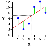
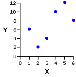
   To illustrate the next point in closer detail, we will focus for a moment on the particular pairing of Xi and Yi values that produced the positive correlation shown in Example II of Figure 7.1.

Pair
Xi
Yi
 
a
b
c
d
e
f
1
2
3
4
5
6
6
2
4
10
12
8


When you perform the computational procedures for linear correlation and regression, what you are essentially doing is defining the straight line that best fits the bivariate distribution of data points, as shown shown in the following version of the same graph. This line is spoken of as the regression line, or line of regression, and the criterion for "best fit" is that the sum of the squared vertical distances (the green lines ||||) between the data points and the regression line must be as small as possible.


As it happens, this line of best fit will in every instance pass through the point at which the mean of X and the mean of Y intersect on the graph. In the present example, the mean of X is 3.5 and the mean of Y is 7.0. Their point of intersection occurs at the convergence of the two dotted gray lines.

   The details of this line—in particular, where it begins on the Y axis and the rate at which it slants either upward or downward—will not be explicitly drawn out until we consider the regression side of correlation and regression. Nonetheless, they are implicitly present when you perform the computational procedures for the correlation side of the coin. As indicated above, the slant of the line upward or downward is what determines the sign of the correlation coefficient (r), positive or negative; and the degree to which the data points are lined up along the line, or scattered away from it, determines the strength of the correlation (r2).

   You have already encountered the general concept of variance for the case where you are describing the variation that exists among the variate instances of a single variable. The measurement of linear correlation requires an extension of this concept to the case where you are describing the co-variation that exists among the paired bivariate instances of two variables, X and Y, together. We have already touched upon the general concept. In positive correlation, high values of X tend to be associated with high values of Y, and low values of X tend to be associated with low values of Y. In negative correlation, it is the opposite: high values of X tend to be associated with low values of Y, and low values of X tend to be associated with high values of Y. In both cases, the phrase "tend to be associated" is another way of saying that the variability in X tends to be coupled with variability in Y, and vice versa—or, in brief, that X and Y tend to vary together. The raw measure of the tendency of two variables, X and Y, to co-vary is a quantity known as the covariance. As it happens, you will not need to be able to calculate the quantity of covariance in and of itself, because the destination we are aiming for, the calculation of r and r2, can be reached by way of a simpler shortcut. However, you will need to have at least the general concept of it; so keep in mind as we proceed through the next few paragraphs that covariance is a measure of the degree to which two variables, X and Y, co-vary.

   In its underlying logic, the Pearson product-moment correlation coefficient comes down to a simple ratio between (i) the amount of covariation between X and Y that is actually observed, and (ii) the amount of covariation that would exist if X and Y had a perfect (100%) positive correlation. Thus

r =
observed covariance
maximum possible positive covariance

   As it turns out, the quantity listed above as "maximum possible positive covariance" is precisely determined by the two separate variances of X and Y. This is for the simple reason that X and Y can co-vary, together, only in the degree that they vary separately. If either of the variables had zero variability (for example, if the values of Xi were all the same), then clearly they could not co-vary. Specifically, the maximum possible positive covariance that can exist between two variables is equal to the geometric mean of the two separate variances.
For any n numerical values, a, b, c, etc., the geometric mean is the nth root of the product of those values. Thus, the geometric mean of a and b would be the square root of axb; the geometric mean of a, b and c would be the cube root of axbxc; and so on.


So the structure of the relationship now comes down to

r =
observed covariance
sqrt[(varianceX) x (varianceY)]

Recall that "sqrt" means "the square root of."

   Although in principle this relationship involves two variances and a covariance, in practice, through the magic of algebraic manipulation, it boils down to something that is computationally much simpler. In the following formulation you will immediately recognize the meaning of SSX, which is the sum of squared deviates for X; by extension, you will also be able to recognize SSY, which is the sum of squared deviates for Y.
In order to get from the formula above to the one below, you will need to recall that the variance (s2) of a set of values is simply the average of the squared deviates: SS/N.


The third item, SCXY, denotes a quantity that we will speak of as the sum of co-deviates; and as you can no doubt surmise from the name, it is something very closely akin to a sum of squared deviates. SSX is the raw measure of the variability among the values of Xi; SSY is the raw measure of the variability among the values of Yi; and SCXY is the raw measure of the co-variability of X and Y together.

r =
SCXY
sqrt[SSX x SSY]


To understand this kinship, recall from Part 4 precisely what is meant by the term "deviate."

   For any particular item in a set of measures of the variable X,
    deviateX=Xi  MX
Similarly, for any particular item in a set of measures of the variable Y,
    deviateY=Yi  MY
As you have probably already guessed, a co-deviate pertaining to a particular pair of XY values involves the deviateX of the Xi member of the pair and the deviateY of the Yi member of the pair. The specific way in which these two are joined to form the co-deviate is

    co-deviateXY = (deviateX) x (deviateY)
And finally, the analogy between a co-deviate and a squared deviate:

For a value of Xi, the squared deviate is
   (deviateX) x (deviateX)
For a value of Yi it is
   (deviateY) x (deviateY)
And for a pair of Xi and Yi values, the co-deviate is
   (deviateX) x (deviateY)


   This should give you a sense of the underlying concepts. Just keep in mind, no matter what particular computational sequence you follow when you calculate the correlation coefficient, that what you are fundamentally calculating is the ratio

r =
observed covariance
maximum possible positive covariance

which, for computational purposes, comes down to

r =
SCXY
sqrt[SSX x SSY]


   Now for the nuts-and-bolts of it. Here, once again, is the particular pairing of Xi and Yi values that produced the positive correlation shown in Example II of Figure 7.1. But now we subject them to a bit of number-crunching, calculating the square of each value of Xi and Yi, along with the cross-product of each XiYi pair. These are the items that will be required for the calculation of the three summary quantities in the above formula: SSX, SSY, and SSXY.

Pair
Xi
Yi
  Xi2 Yi2   XiYi  
a
b
c
d
e
f
1
2
3
4
5
6
6
2
4
10
12
8
1
4
9
16
25
36
36
4
16
100
144
64
6
4
12
40
60
48
sums
21
42
91
364
170

SSX : sum of squared deviates for Xi valuesT
   You saw in Part 4 that the sum of squared deviates for a set of Xi values can be calculated according to the computational formulaT
   
In the present example,
   N=6  [because there are 6 values of Xi]
   Xi2 = 91
   Xi = 21
   (Xi)2 = (21)2 = 441
Thus:
   SSX = 91(441/6) = 17.5
SSY : sum of squared deviates for Yi valuesT
   Similarly, the sum of squared deviates for a set of Yi values can be calculated according to the formulaT
   
In the present example,T
   N = 6  [because there are 6 values of Yi]
   Yi2 = 364
   Yi = 42
   (Yi)2 = (42)2 = 1764
Thus:
   SSY = 364(1764/6) = 70.0
SCXY : sum of co-deviates for paired values of Xi and YiT
   A moment ago we observed that the sum of co-deviates for paired values of Xi and Yi is analogous to the sum of squared deviates for either of those variables separately. You will probably be able to see that this analogy also extends to the computational formula for the sum of co-deviates:T

Again, for the present example,T
   N = 6  [because there are 6 XiYi pairs]
   Xi = 21
   Yi = 42
   (Xi)(Yi) = 21 x 42 = 882
   (XiYi) = 170
Thus:
   SCXY = 170(882/6) = 23.0

Once you have these preliminaries,T
   SSX = 17.5, SSY = 70.0, and SCXY = 23.0
you can then easily calculate the correlation coefficient as

r =
SCXY
sqrt[SSX x SSY]
 
=
23.0
sqrt[17.5 x 70.0]
= +0.66

and the coefficient of determination as

r2 = (+0.66)2 = 0.44

   To make sure you have a solid grasp of these matters, please take a moment to work your way through the details of Table 3.1, which will show the data and calculations for each of the examples of Figure 7.1. Recall that each example starts out with the same values of Xi and Yi; they differ only with respect to how these values are paired up with one another.

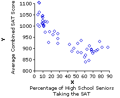
   Larger, more complex data sets will of course require something more laborious—but the general principles and specific computational procedures are precisely the same, either way. Consider, for example, the data set we referred to at the beginning of Part 6, pertaining to the correlation between the percentage of high school seniors taking the SAT versus average state score on the SAT.


   Table 3.2 shows the details of calculation for this data set. As you will see, it requires quite a large number of separate operations, many of which result in multi-digit numerical values. There was a time in the not too distant past when students of statistics had to perform calculations of this sort armed with nothing but paper, pencil, and patience, and it was a very laborious enterprise indeed. But that was then, and this is now. With a fairly inexpensive pocket calculator and a little practice in using it to its full advantage, you can perform complex calculations of this sort with a speed that would have made an earlier generation of statistics students weep with envy. With a computer spreadsheet, and again a little practice, you can do it even faster. With pre-packaged computer software, such as the linear correlation page on the VassarStats website, you can do it with as little time and effort as it takes you to enter the paired values of Xi and Yi.

   At any rate, once you perform the operations required to arrive at the following sums (from Table 3.2), all the rest is simple and straightforward:

Sums of
Xi
Yi
  Xi2
Yi2
  XiYi
 1,816 
 47,627 
 102,722 
 45,598,101 
 1,650,185 

Given these results from the preliminary number-crunching, you could then (as shown in Table 3.2) easily calculate

    SSX = 36,764.88

    SSY = 231,478.42

    SCXY = 79,672.64

    r = 0.86

    r2 = 0.74


Go to Part 8 [The Interpretation of Correlation]